Published:
Michael Phillips, Lunar and Planetary Laboratory, University of Arizona
This is a working paper posted as a blog post; it has not been peer reviewed. The code, an interactive map explorer, and the data archive are openly available. The section “How this was made” near the end describes how the paper was written with Claude, an AI model made by Anthropic.
Abstract
We compiled crater-on-crater superposition relations among all cataloged impact craters on Mars into a single directed graph, in which each edge records that one crater formed after another. Nodes are the 385,049 craters ≥1 km in diameter in the Robbins and Hynek (2012) database. A crater lying entirely inside another crater’s rim is assigned as the younger of the pair. Pairs whose rims cross are oriented by two independent tests: the fraction of each rim traced in Thermal Emission Imaging System (THEMIS) daytime infrared mosaics, and rim continuity measured on Mars Orbiter Laser Altimeter (MOLA) topography. The graph links 83,370 craters through 77,661 relations (73,183 after transitive reduction) and contains no cycles. The two rim-overlap tests agree on 98.1% of the 1,021 pairs that both resolve. Edges oriented by the rim-arc test agree with rim degradation classes in 90.0% of testable pairs, which matches the 89.8% agreement of geometrically certain containment edges. A blind visual check on Context Camera (CTX) images matched the graph for 38 of 40 pairs. The fraction of craters linked into the graph, and the length of superposition chains, both increase with crater diameter and with the age of the host geologic unit.
We then use the graph to test crater-count ages and to measure how craters are erased. For 3,419 linked pairs of craters 10–600 km across, the older crater’s interior holds 1.66 times the crater density of the younger crater’s interior. Counts of 1–2 km craters reverse the superposition order for 16% of pairs, against 3% for larger craters, so interior ages measured with small craters record later resurfacing. Stacked interior counts place rim degradation classes 1 to 4 at 3.78, 3.75, 3.62, and 3.32 Ga. A Bayesian sequence model combines the counts with the order and is calibrated on synthetic sequences. Superposition chains are at most four relations deep. A Monte Carlo cratering model reproduces the observed chain depths to within about 30% when craters degrade diffusively at about 1×10⁵ m²/Myr before 3.7 Ga and at no more than 10 m²/Myr afterward, and when a crater leaves the record once later impacts have removed 30% of its rim. These rates correspond to 0.7–2.8 m/Myr of crater depth loss in the Noachian and less than 3 nm/yr since, consistent with published estimates. The graph, the code, and an interactive map explorer are openly available.
1. Introduction
Superposition is the most direct evidence of relative age on a cratered surface. Shoemaker and Hackman (1962) used it to build the first lunar time scale, ordering craters and basins by which ejecta and rays lay on top of which. The Martian stratigraphic system rests on the same observations combined with crater densities (Tanaka, 1986; Tanaka et al., 2014). Crater size-frequency distributions give model ages for surfaces (Hartmann and Neukum, 2001; Michael and Neukum, 2010), but they do not order the individual craters on a surface.
Superposition relations between individual craters are recorded in geologic maps and in studies of particular basin sequences (Wilhelms, 1987; Fassett et al., 2012). Each of those records covers one map area or one set of features. A global crater catalog makes a planet-wide compilation possible, because the geometry of two cataloged rims, together with a test of which rim survives where they meet, decides which crater formed first.
Archaeologists record the same kind of information in a Harris matrix, in which each stratigraphic unit is a node and each direct superposition links a later unit to an earlier one (Harris, 1979). The result is a directed acyclic graph whose partial order is the stratigraphic sequence. We apply that structure to Martian craters. Each crater in the Robbins and Hynek (2012) database is a node, and each edge points from an older crater to a younger crater that cuts it or sits inside it.
A graph of this kind supports four uses. It gives each crater ordinal age constraints from its neighbors, it provides an independent check on degradation classes and model ages, it supplies labeled examples for image-based classifiers, and it gives the crater sequence for any region directly. This paper describes the first version of the graph, the tests used to orient its edges, and its validation. It then applies the graph to three questions: whether crater-count ages agree with superposition order, why superposition chains are short, and how fast Martian craters degraded.
2. Data
Crater catalog. We used the 2020 public release of the Robbins and Hynek (2012) database, which lists 385,049 craters ≥1 km in diameter. Rims were traced on the THEMIS daytime infrared global mosaic at ~100 m/pixel (Christensen et al., 2004; Edwards et al., 2011) and fit with circles. We used each crater’s circle-fit center and diameter, the fraction of the rim arc that could be traced (ARC_IMG), the rim degradation class (DEG_RIM, 1 = most degraded to 4 = freshest; assigned to 74,164 craters, including 93% of craters ≥3 km), and the ejecta morphology. Layered ejecta, in the nomenclature of Barlow et al. (2000), are mapped for 19,744 craters.
Topography. We used the MOLA Mission Experiment Gridded Data Records at 128 pixels/degree (~463 m/pixel at the equator) between 88°N and 88°S (Smith et al., 2001).
Geologic units. Each crater center was assigned to a unit of the global geologic map of Mars (Tanaka et al., 2014). We record the oldest period in the unit name (Noachian, Hesperian, or Amazonian) as the host-unit period. On this basis 253,519 cataloged craters sit on Noachian units, 121,330 on Hesperian units, and 10,200 on Amazonian units.
Validation imagery. The global CTX mosaic at ~5 m/pixel (Malin et al., 2007; Dickson et al., 2024) was used only to check edge orientations visually, within 296–336°E and 28–68°S.
3. Method
3.1 Candidate pairs
For each crater we found every smaller crater whose center lies within three radii of its own center, using a k-d tree on unit vectors and great-circle distances on a sphere of radius 3,389.5 km. For a pair with larger radius r_l, smaller radius r_s, and center separation d, the two rim circles fall into one of four classes (Table 1). Only the first two classes yield edges in this version.
Table 1. Pair classes, counts, and outcomes.
| Class | Geometry | Pairs | Edges in the graph |
|---|---|---|---|
| Containment | d + r_s ≤ r_l | 61,998 | 61,975 |
| Rim overlap | rims cross, (r_l + r_s − d) ≥ 0.1 r_s | 26,711 | 15,686 |
| Marginal overlap | rims cross, (r_l + r_s − d) < 0.1 r_s | 2,778 | none |
| Ejecta zone | r_l + r_s ≤ d < 2r_l + r_s | 291,097 | none |
3.2 Containment
A crater lying entirely inside another crater’s rim is younger, because the larger impact would have excavated or buried any crater already inside its rim. We treat these edges as certain, with two exceptions. Five pairs of nearly coincident circles (d < 0.15 r_l and r_s/r_l > 0.9) are duplicate catalog entries and were removed. Eighteen large nested pairs with nearly common centers (d < 0.2 r_l, 0.3 ≤ r_s/r_l ≤ 0.9, and r_s ≥ 10 km) more likely trace the inner ring of one basin, so we set them aside.
3.3 Rim overlap: rim-arc completeness
Where two rims cross, the younger rim is continuous and the older rim is missing inside the younger crater. The catalog records this directly, because ARC_IMG is the fraction of each rim that could be traced. For crater k with a fraction f_k of its rim circle inside its partner, we define a youth index:
An intact rim gives y_k = 1, and a rim missing exactly where the partner sits gives y_k = 0. The index is defined only for f_k ≥ 0.1. The test calls the smaller crater younger when y_s − y_l ≥ 0.5, treating an undefined y_l as 0.5. It calls the larger crater younger only when both indices are defined and y_l − y_s ≥ 0.5. One-sided calls of the second kind agreed with degradation classes in 70% of testable pairs during development, so we excluded them.
3.4 Rim overlap: rim continuity on topography
The second test measures the same property on MOLA topography (Figure 1). For each crater of radius r we sample elevation h along 72–720 azimuths θ, spaced at most half a pixel apart on the rim, and compute rim prominence:
\[p(\theta) = \max_{0.85 \le \rho \le 1.15} h(\rho r, \theta) - \tfrac{1}{2}\left[h(0.7r, \theta) + h(1.35r, \theta)\right]\]A uniform slope or a concave crater floor along the profile can raise p by at most 27% of the elevation difference between the 0.7 r and 1.35 r samples, so a large positive p marks a surviving ridge. The intrusion arc A_in is the set of rim points less than 0.85 r from the partner’s center, and the reference arc A_ref is the set more than 1.25 r away. The preservation ratio is:
\[P = \frac{\operatorname{median}_{\theta \in A_{\mathrm{in}}} p(\theta)}{\operatorname{median}_{\theta \in A_{\mathrm{ref}}} p(\theta)}\]We require at least three azimuths on each arc and a reference prominence of at least 15 m. A rim with P ≥ 0.6 is intact, and a rim with P ≤ 0.25 is breached. The test orients a pair when one rim is intact and the other is breached, and only when the smaller crater is at least 3 km across (~6.5 MOLA pixels).
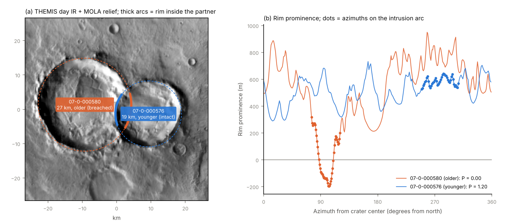
Figure 1. Rim-continuity test on craters 07-0-000580 (27 km) and 07-0-000576 (19 km) at 9.3°S, 346.9°E. (a) THEMIS daytime infrared mosaic blended with MOLA shaded relief, with the rim circles; thick arcs mark each rim inside its partner. (b) Rim prominence against azimuth. On the intrusion arc (dots) the larger crater’s rim drops below zero (P = 0.00), while the smaller crater’s rim keeps its prominence (P = 1.20). The rim-arc test agrees that the smaller crater is younger.
3.5 Combining the tests and building the graph
An overlap edge receives high confidence when both tests orient it the same way (1,002 edges) and medium confidence when the rim-arc test decides alone (14,684 edges). Edges decided by topography alone (496) are kept at low confidence and excluded from the default graph, for the reason given in Section 4. The 19 pairs on which the tests disagree, and 10,510 pairs that neither test decides, stay unoriented.
Edges point from the older crater to the younger crater. We searched the graph for strongly connected components, which would mark contradictory cycles, and computed its transitive reduction (Aho et al., 1972) with NetworkX (Hagberg et al., 2008). For each crater we report its depth (the longest chain of older craters beneath it), its height (the longest chain of younger craters above it), the number of craters known to be older and younger, and its weakly connected component.
4. Validation
Four checks test the edge orientations against independent evidence (Table 2). Together they give rim-arc edges an implied accuracy of 94% or higher in every size class tested, and they show that topography-only edges are not reliable enough for the default graph.
Table 2. Agreement of inferred orientations with independent evidence.
| Check | Pairs | Agreement |
|---|---|---|
| Containment edges vs. degradation class (reference ceiling) | 5,452 | 89.8% |
| Rim-arc + topography edges vs. degradation class | 646 | 95.4% |
| Rim-arc edges vs. degradation class | 3,019 | 90.0% |
| Topography-only edges vs. degradation class (excluded) | 222 | 73.4% |
| Rim-arc test vs. topography test | 1,021 | 98.1% |
| Blind visual check on CTX, edges in the graph | 40 | 95.0% |
| Younger crater is the one with layered ejecta | 2,150 | 66.1% |
Degradation classes. A fresher rim class suggests a younger crater, but degradation also depends on size, target, and local resurfacing. We therefore measured how often the class agrees with containment edges, whose direction is fixed by geometry. Among containment pairs with different rim classes, the inner crater has the fresher rim in 89.8% of cases, and this value q is the agreement a perfectly oriented edge set would reach. For an edge set with observed agreement A, and assuming degradation-class errors are independent of the method, the implied fraction of correctly oriented edges is:
\[a = \frac{A - (1 - q)}{2q - 1}\]Rim-arc edges (A = 0.900) and edges confirmed by both tests (A = 0.954) reach or exceed the ceiling, which gives a ≈ 1. By size of the smaller crater, rim-arc edges give a = 0.97 for 10–20 km and a = 0.94 for craters ≥20 km. Topography-only edges give a = 0.79, which is why we excluded them. Containment pairs and overlap pairs differ in size contrast, so the independence assumption is approximate.
Cross-agreement. The rim-arc test uses rim tracing on THEMIS images, and the rim-continuity test uses MOLA elevations. Where both reach a decision, they agree on 98.1% of 1,021 pairs.
Blind visual check. We drew 82 pairs at random within the CTX coverage listed in Section 2, stratified by method and by size of the smaller crater. Each pair was rendered with its two circles labeled A and B in random order, and the younger crater was judged from the image before the labels were matched to the graph. Forty-six pairs could be judged; the rest fell on data gaps, low-resolution fill, or ambiguous morphology. The graph matched the visual call for 38 of the 40 judgeable pairs whose edges are in the default graph, including 19 of 21 pairs with a smaller crater under 3 km. Both mismatches involve craters smaller than 2.5 km. In this draft the visual calls were made by the AI assistant that wrote the pipeline (see Acknowledgments), and a repeat by human reviewers is planned.
Layered ejecta. In the catalog, layered ejecta are mapped for 54% of craters in the freshest rim class and 2% of craters in the most degraded class, so preserved layered ejecta mark relatively young craters. When exactly one crater of an oriented pair has mapped layered ejecta, that crater is the younger one in 66.1% of 2,150 pairs. This check is weak, but its sign agrees with the others.
The default graph contains no cycles. Cycles would arise if some edges contradicted others along a closed loop, so their absence is a further consistency check, although most of the graph is tree-like and offers few opportunities for contradiction.
5. Results
The default graph links 83,370 of the 385,049 cataloged craters (21.7%) through 77,661 edges, of which 61,975 come from containment and 15,686 from rim overlap. Transitive reduction removes 4,478 edges that are implied by longer chains, leaving 73,183 direct relations. Figure 2 shows where the linked craters lie.
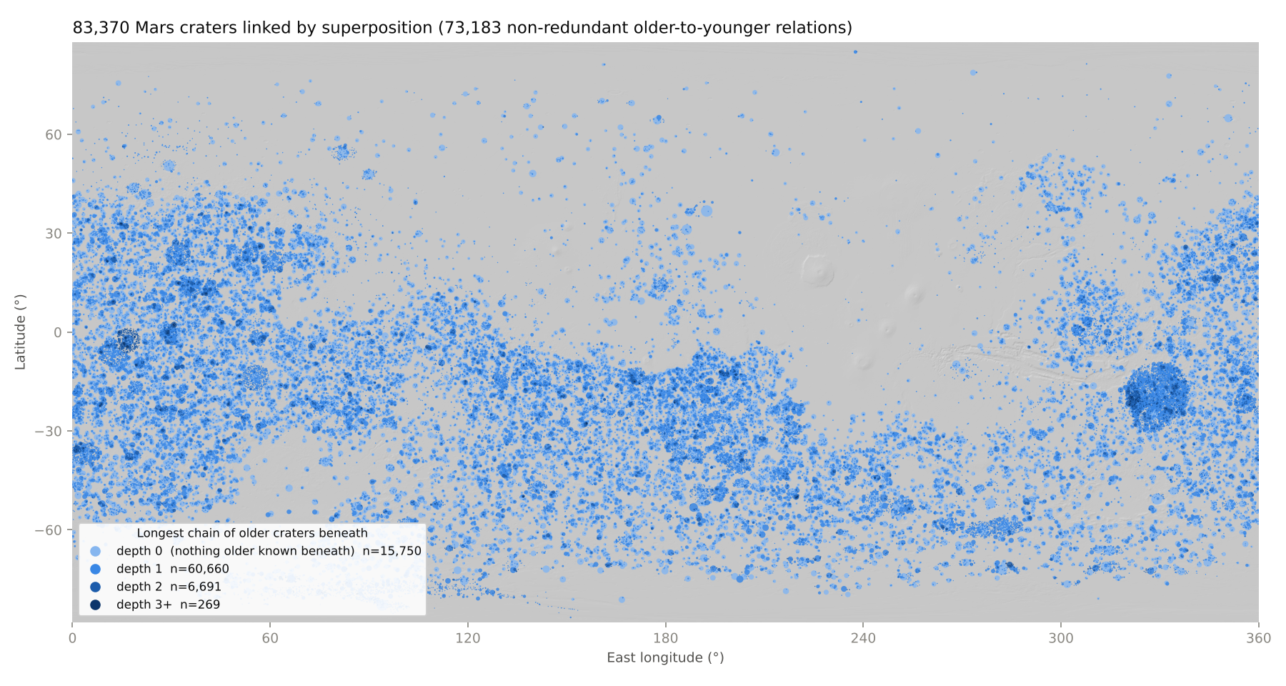
Figure 2. Craters in the default graph on MOLA shaded relief, colored by depth (the longest chain of older craters beneath each crater) and sized by diameter.
Clusters. Craters that never touch cannot be ordered by superposition, so the graph splits into 14,415 weakly connected clusters. The median cluster holds 2 craters, and 83% of clusters hold 5 or fewer. The 52 clusters with at least 100 craters hold 19,889 craters between them. Each large cluster is organized around one large crater and the craters inside it. The largest, with 6,146 craters, belongs to the 1,088 km crater 07-4-043926 centered at 18.2°S, 329.4°E.
Chain depth. Of the linked craters, 15,750 have no known older crater beneath them (depth 0), 60,660 have depth 1, 6,691 depth 2, 266 depth 3, and 3 depth 4. The longest chains contain 5 craters. In one example, the 625 km crater 07-4-043925 contains the 37 km crater 07-1-014021, which contains the 1.6 km crater 07-4-019699; two successively younger craters of 1.6 and 1.3 km then cut that crater’s rim.
Dependence on size and terrain age. The fraction of craters linked into the graph rises with diameter on every host-unit period (Figure 3). Between 83% and 99.7% of craters ≥50 km are linked, depending on the host-unit period, because most of them contain at least one smaller cataloged crater. At every diameter, craters on Noachian units are linked more often than craters on Hesperian units, which in turn are linked more often than craters on Amazonian units. Long chains follow the same order: depth ≥2 applies to 8.6% of linked craters on Noachian units, 7.4% on Hesperian units, and 1.1% on Amazonian units. This ordering is expected, because older units carry higher crater densities (Tanaka et al., 2014) and therefore more overlapping craters.
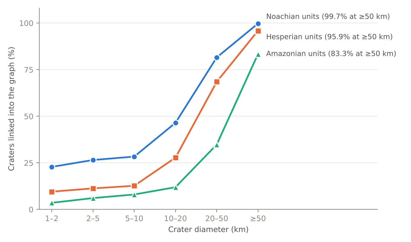
Figure 3. Fraction of cataloged craters linked into the default graph, by diameter and by the period of the host geologic unit.
A regional example. Figure 4 shows the transitive reduction for a 4° by 5° area of Noachian highlands near 35.5°S, 1°E. The 125 km crater 11-1-016542 contains the 55 km crater 11-0-000806 and 54 of the smaller craters in view, and it lies inside the 425 km crater 11-0-000000 beyond the map edge. Rim-overlap edges (11 of the 96 shown) order neighboring craters whose rims cross.
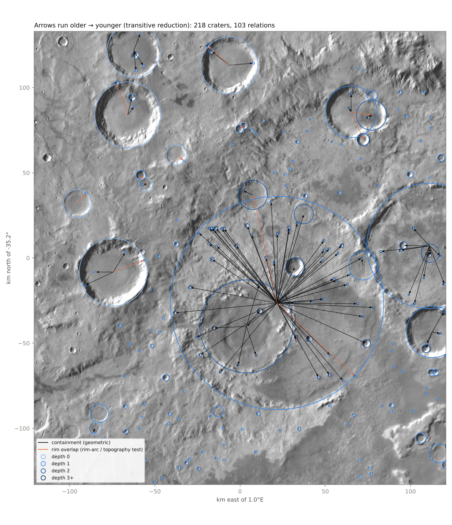
Figure 4. Transitive reduction of the graph for 33.0–37.5°S, 358.5°E–3.5°E on THEMIS daytime infrared blended with MOLA shaded relief. Arrows run from older to younger craters; black arrows are containment edges and orange arrows are rim-overlap edges. Circle shading gives depth as in Figure 2.
Connections per crater. Most linked craters have a single relation: 65,621 of the 83,370, or 79%. Only 1,144 craters have 10 or more relations, 49 have 100 or more, and four have more than 1,000 (Figure 5). All four are large basins, and the 1,088 km crater 07-4-043926, which matches the position of Ladon basin near 18°S, 330°E, has 5,694. Between 100 and 1,000 relations the cumulative count falls as a power law with a slope near −1.1. The tail is inherited from crater sizes. Nearly all of a crater’s relations are younger craters inside it, and their mean number rises as D^2.16 for craters ≥16 km. Martian craters larger than about 40 km have a cumulative size distribution with a slope near −2.5, which predicts a slope of −2.5/2.16 ≈ −1.15 for the number of relations. The 07-4-043926 basin and the 471 km crater 07-3-000215 inside it probably trace the outer and inner rings of Ladon; the pipeline flags the pair as a possible basin ring and draws no edge between them. No crater has more than five older neighbors, and Section 8 compares these counts with a cratering model.
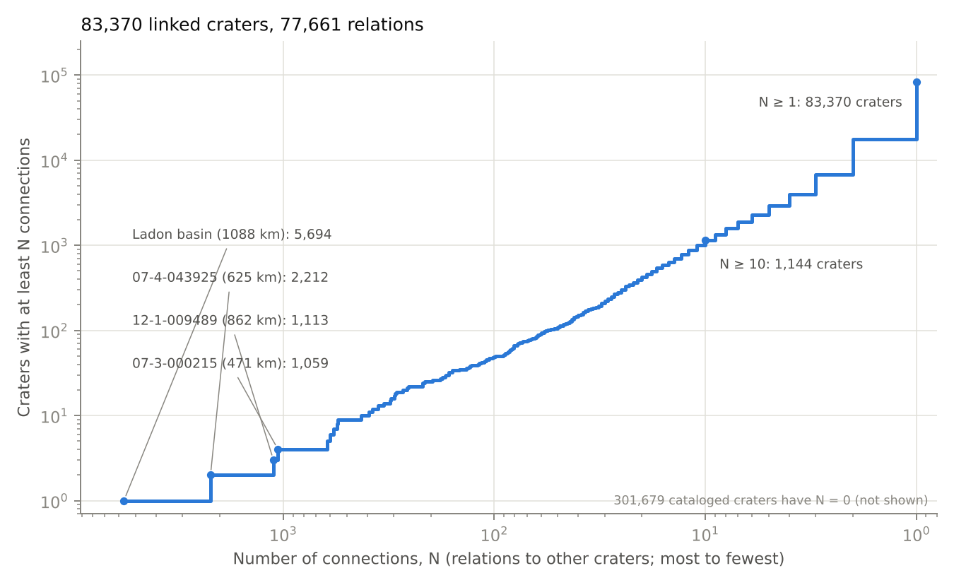
Figure 5. Number of craters with at least N relations to other craters, with N decreasing to the right, on logarithmic axes. The four most connected craters are labeled. The 301,679 cataloged craters with no relation are not shown.
6. Crater-count ages and superposition order
Superposition order is independent of crater statistics, so it can test crater-count ages one crater at a time. We compared the interior crater densities of the 24,382 craters 10–600 km across with the order the graph gives them, and then combined the two.
6.1 Interior counts in crater time
We express age as crater time, τ: the cumulative density of craters ≥1 km (N(1), per km²) that a surface has accumulated since it formed. With a spatially uniform flux and a production function of fixed shape, craters arrive at a constant rate in τ whatever the impact-rate history. Superposition order is unchanged by any monotonic mapping from τ to years, so this comparison tests crater counting, the production function, and resurfacing, but not the absolute chronology. Model ages use the production function of Ivanov (2001), the chronology function of Hartmann and Neukum (2001), and the epoch boundaries of Michael (2013), with coefficients as distributed in craterstats (Michael and Neukum, 2010).
For each host crater we counted the craters whose centers lie inside its rim. A crater of diameter D can be recorded only where no larger younger crater has since excavated the surface. The count area for diameter D, A_eff(D), therefore excludes the interiors of larger superposed craters, and a crater is counted only if it does not itself lie inside a larger superposed crater (Kneissl et al., 2016). We also excluded younger craters that overlap the rim from outside, flagged duplicates and basin rings, and craters that the graph places older than the host. With the production function’s shape fixed, the count k of craters ≥D_min is a sufficient statistic for τ:
\[k \sim \mathrm{Poisson}(\tau\,\Lambda), \qquad \Lambda = \int_{D_{\min}}^{D_{\mathrm{host}}} f(D)\,A_{\mathrm{eff}}(D)\,dD\]Here f is the differential production function normalized to N(1) = 1.
6.2 Interior densities agree with superposition order
The older crater of a graph edge has the denser interior. Of the 3,835 edges between two host craters, 3,419 have at least one counted crater ≥1 km. Across these edges the older interior holds 1.66 times (95% interval 1.58–1.73) the crater density of the younger interior, and 1.82 times (1.57–1.99) when only craters ≥3 km are counted (Figure 6b). Given the total count k on the two interiors, the older crater’s share is binomial with probability ρΛ_old/(ρΛ_old + Λ_young), where ρ = τ_old/τ_young. We modeled log ρ across edges as normal, integrated out the counting noise, fit by maximum likelihood, and bootstrapped over edges (200 resamples). In 1,934 edges the younger crater lies inside the older crater’s count area. That crater defines the edge, so we removed it from the older crater’s count.
Table 3. Interior density ratio (older ÷ younger) and estimated fraction of edges with the older crater’s interior sparser, by edge type.
| Edge type | Edges (D_min = 1 km) | Ratio, ≥1 km | Ratio, ≥3 km | Inverted, ≥1 km | Inverted, ≥3 km |
|---|---|---|---|---|---|
| Containment | 1,298 | 1.84 | 2.03 | 8.6% | 3.8% |
| Rim overlap, rim-arc test | 1,534 | 1.60 | 2.01 | 15.2% | 0.0% |
| Rim overlap, both tests | 587 | 1.57 | 1.56 | 15.0% | 12.0% |
Containment and rim-arc edges converge on a ratio near 2 at D_min = 3 km. Edges decided by both rim tests stay 12–16% inverted at every D_min; these pairs are larger and closer in density, and we have not separated near-coeval pairs from order errors among them. Robbins et al. (2013) found model ages consistent with superposition for a handful of overlapping craters ≥150 km, and Fassett et al. (2012) found the same for the sequence of lunar basins. This test extends that comparison to thousands of crater pairs 10–600 km across.
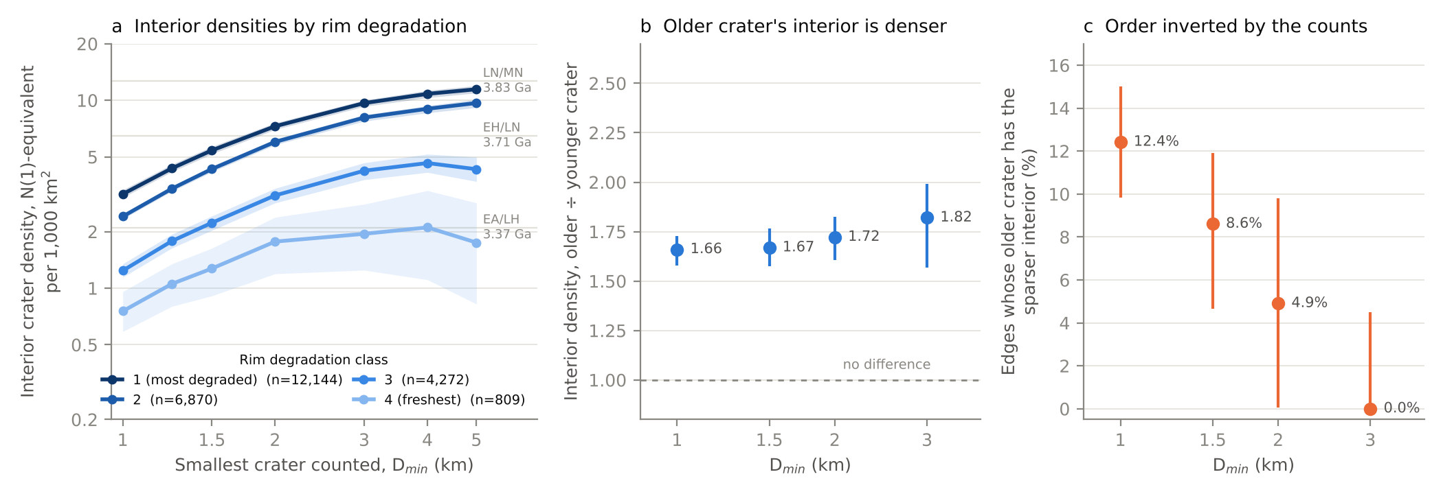
Figure 6. (a) Stacked interior crater density against the smallest diameter counted, by rim degradation class, for craters 10–600 km; bands are 95% bootstrap intervals and gray lines mark epoch boundaries (Michael, 2013). (b) Typical ratio of older to younger interior density across graph edges, with 95% bootstrap intervals. (c) Estimated fraction of edges whose older crater has the sparser interior.
6.3 Small craters record resurfacing
Interior model ages measured with small craters are retention ages. Under a fixed production function, the N(1)-equivalent density of an interior should not depend on the smallest diameter counted. Instead, stacked interior densities rise 3.5–4.0 times from D_min = 1 km to D_min = 5 km for rim degradation classes 1–3, and 2.3 times for class 4 (Figure 6a). The estimated fraction of edges whose older crater has the sparser interior falls from 12.4% (95% interval 9.8–15.0%) at D_min = 1 km to at most 4.5% at D_min = 3 km (Figure 6c).
Craters 1–2 km and craters ≥2 km are disjoint samples of each interior. A bivariate normal fit to the two density ratios across 2,717 edges gives 16% of edges inverted by the 1–2 km craters and 3% inverted by the larger craters. For 11% of edges the small craters invert the order while the larger craters on the same interiors keep it, which identifies interiors resurfaced after a younger crater formed beside or inside them. Robbins et al. (2013) found the same diameter dependence on the rims of large craters and did not count on crater floors for this reason.
Stacked counts of craters ≥3 km give a model age for each rim degradation class (Table 4).
Table 4. Stacked interior model ages by rim degradation class, craters 10–600 km, counting craters ≥3 km. Intervals cover counting noise only.
| Rim degradation class | Craters | Model age (Ga) | 95% interval (Ga) |
|---|---|---|---|
| 1 (most degraded) | 12,144 | 3.78 | 3.78–3.79 |
| 2 | 6,870 | 3.75 | 3.74–3.76 |
| 3 | 4,272 | 3.62 | 3.59–3.64 |
| 4 (freshest) | 809 | 3.32 | 2.56–3.50 |
Classes 1 and 2 fall in the Late Noachian, class 3 in the Early Hesperian, and class 4 near the Hesperian–Amazonian boundary. The step between classes 2 and 3 matches the transition near 3.7 Ga that Mangold et al. (2012) dated from 283 craters >20 km in two highland regions. Because the ages are interior retention ages, each is a minimum for its class.
6.4 A Bayesian sequence model
Interior counts alone cannot order most crater pairs. The graph orders 3,933 pairs of host craters. With counts of craters ≥3 km and a population prior, the mean probability of the wrong order across those pairs is 0.37, and 903 pairs (23%) are placed in the wrong order more likely than not. Only 875 host craters have three or more counted craters ≥3 km, and their median diameter is 80 km.
We therefore combined the counts with the order, following Bayesian chronological models of archaeological sequences (Buck et al., 1991; Bronk Ramsey, 2009). Each crater has a formation crater time τ and a Poisson likelihood from its interior count (D_min = 3 km). Craters with no older neighbor take the population distribution of formation crater times, estimated from all host craters by empirical Bayes on a 400-point logarithmic grid. A crater that superposes others formed after all of them. With impacts arriving at a constant rate in crater time, its prior is uniform between zero and the smallest τ of those craters. This impact-arrival prior keeps a host crater with many uninformative superposed craters from being pushed toward old ages, the problem that the uniform-phase prior addresses in radiocarbon sequence models. The order constraints couple 5,822 craters in 2,108 clusters through 3,728 relations after transitive reduction; the longest chain has three relations. A Gibbs sampler updates one color class of the constraint graph at a time (4,000 sweeps after 600 burn-in), and the other 18,560 craters keep closed-form posteriors.
On 700 synthetic clusters of 2–7 craters generated by the same arrival process, the 68% and 95% posterior intervals contain the true τ for 67% and 94% of craters. Independent population priors on the same clusters give 68% intervals that contain the truth for only 63% of craters.
Copernicus crater (302 km in the catalog; 49°S, 169°W) holds 33 craters ≥3 km and has a model age of 3.73 Ga (68% interval 3.70–3.77 Ga) with or without the order (Figure 7). Counts alone place its seven superposed craters ≥10 km at 3.73–3.77 Ga, with upper 68% limits of 3.83–3.85 Ga, older than Copernicus itself. The sequence model bounds them by Copernicus (upper 68% limits 3.70–3.72 Ga) and lets their intervals extend to younger ages.
We count a crater as individually dated when its 68% interval in τ is at most half as wide as the population prior’s. Counts alone date 164 craters, and counts with the order date 202 (41 gained, 3 lost). The gain is 21% with D_min = 2 km (275 to 334) and 21% with a 10% resurfaced-interior mixture in the likelihood (121 to 146). With a catalog complete to 1 km, the model’s main effect is to keep ages consistent with the order; it narrows few intervals.
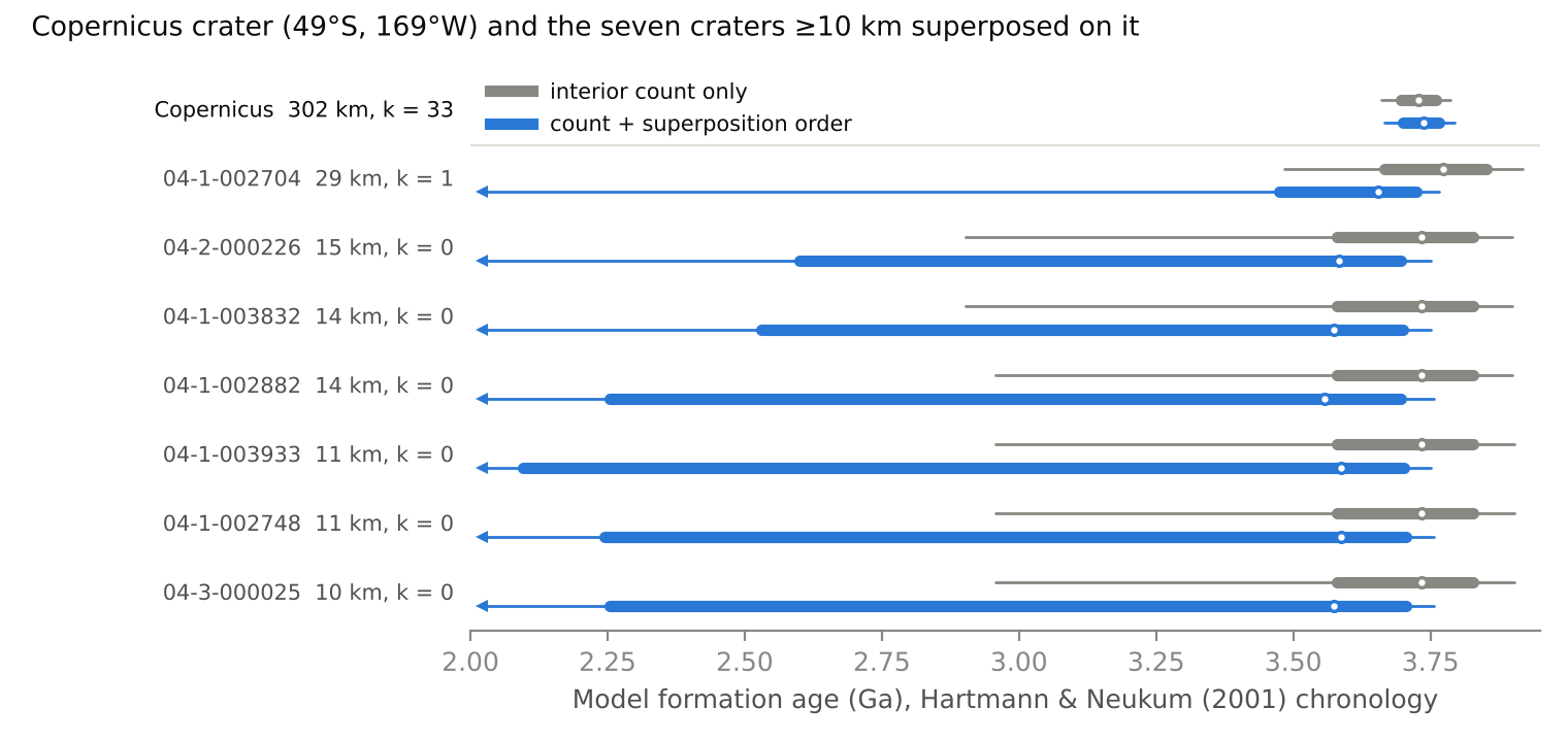
Figure 7. Model formation ages for Copernicus crater and the seven craters ≥10 km superposed on it; k is the number of counted craters ≥3 km. Gray: interior count with the population prior. Blue: the sequence model. Bars show 68% and 95% intervals; arrows mark intervals that continue to younger ages. Chronology of Hartmann and Neukum (2001).
7. Why superposition chains are short
Only 266 linked craters sit at depth 3 and 3 at depth 4 (Section 5). A crater at depth L needs a chain of L older craters beneath it, nested or overlapping, and each crater in the chain must have formed after the one beneath it; a crater that formed first would have been erased by the later impact. In a nested chain each crater must also be smaller than the one containing it. Under random impacts, the time ordering contributes a factor 1/L!, and the size ordering contributes another factorial. For a production function with a cumulative slope near −2, the expected number of craters at depth L + 1 relative to depth L is then about Λ/(L(L + 1)), where Λ is the fraction of a host’s area covered by craters smaller than the host. At the crater density of Noachian units, craters 2–16 km cover about 5% of the surface, which predicts a ratio near 0.025 between nested chains of depth 2 and depth 1. The observed ratio on Noachian units, for craters ≤362 km, is 0.018.
Rim overlaps need no size ordering and have a larger cross section, so they carry most of the deep chains. On Noachian units, containment edges alone place 703 craters at depth 2, against 4,416 with all edges.
Cratering simulation. To test whether random cratering explains the observed depths, we placed craters ≥1 km at random on a periodic patch with the area of the Noachian units (6.8×10⁷ km²), with diameters drawn from the Ivanov (2001) production function between 1 and 362 km. A later crater erases an older one in three ways: when the older crater’s center lies inside the later, larger rim; when the later crater’s ejecta, with thickness following McGetchin et al. (1973), is at least as thick as the older crater is deep; or when later craters together have removed a set fraction of the older crater’s rim. We built the graph from the surviving craters with the pipeline’s geometric rules, took the snapshot at which craters ≥16 km match the Noachian density, and ran three realizations. Monte Carlo models of cratered terrain have long been used to study crater saturation (e.g., Richardson, 2009); here the model is used to predict graph statistics.
Impacts alone produce chains up to six relations deep when every relation is recorded (Figure 8). Nested chains match the observations once the record is thinned to the observed size distribution, removing the oldest craters first: the model gives 600–630 craters at depth 2 against 703 observed. Their scarcity is built into how impacts accumulate, because the unthinned record is just as shallow in nested chains. With the pipeline’s overlap-decision rates applied and craters erased at 50% rim loss, the model still gives 417–472 craters at depth 3 against 152 observed, and 13–21 at depth 4 against 2. Section 8 shows that a 30% rim-loss threshold removes this excess.
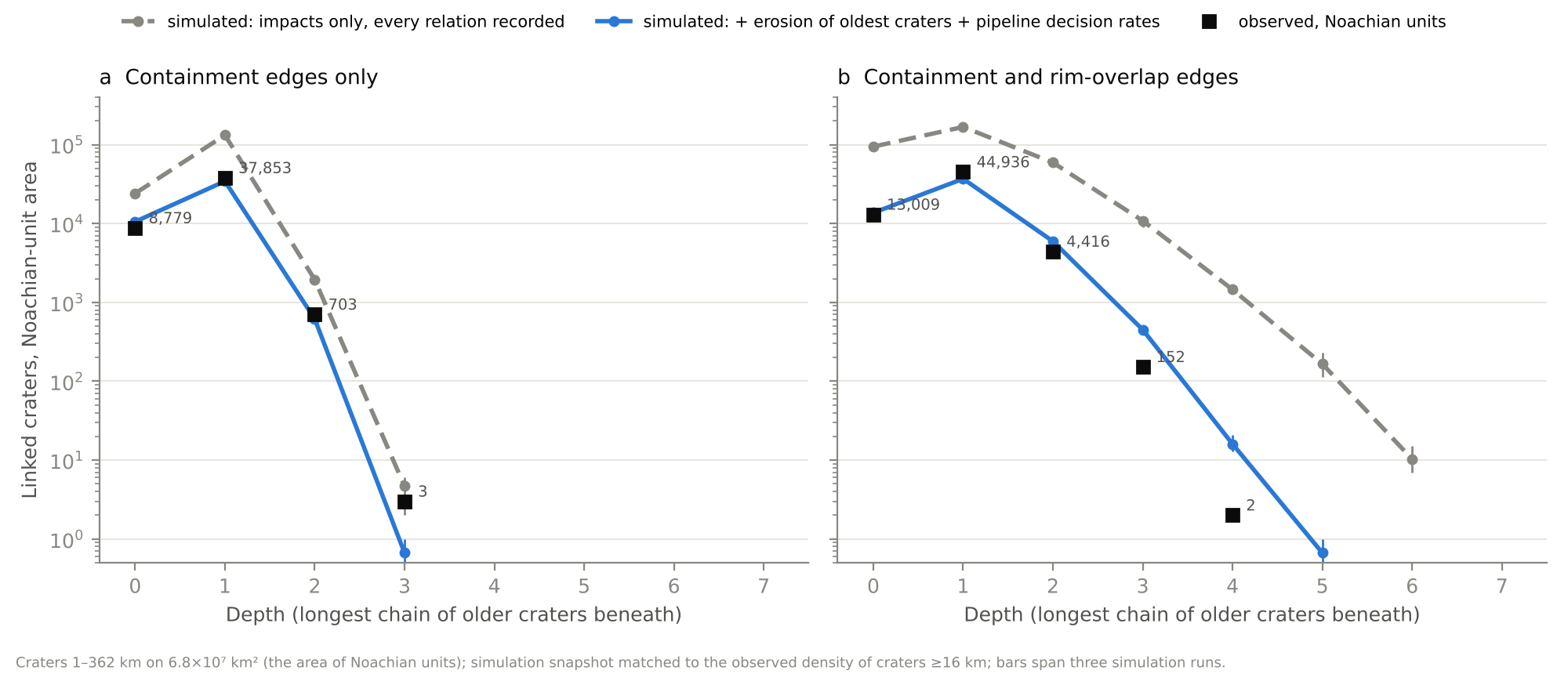
Figure 8. Chain depth on Noachian terrain, observed and simulated, for craters 1–362 km. (a) Containment edges only. (b) Containment and rim-overlap edges. Gray dashed: impacts only, every relation recorded. Blue: record thinned to the observed size distribution by removing the oldest craters first, with the pipeline’s overlap-decision rates. Craters are erased at 50% rim loss. Bars span three realizations.
Chains on Hesperian units. Depth ≥2 applies to 8.6% of linked craters on Noachian units and 7.4% on Hesperian units (Section 5), although Hesperian units hold about one quarter of the Noachian density of craters ≥16 km. Deep chains on Hesperian units sit inside large old craters. For craters at depth ≥2, the largest crater at the base of the chain has a median diameter of 198 km on Hesperian units, against 89 km on Noachian units. For 443 of the 1,037 craters at depth ≥2 on Hesperian units (43%), that base crater is centered on a Noachian unit. These chains start in large craters, many of them older than the Hesperian surfaces around them.
8. Crater degradation rates
The thinning step in Section 7 stands in for erosion and infill. In this section we replace it with a degradation model, fit the model’s two rates to the sizes and depths of craters on Noachian units, and then use the graph to test the fit. Chain depth and the number of older neighbors are not part of the fit.
Degradation model. A fresh crater has depth d₀ = min(0.2D, 0.28D^0.51), with d₀ and D in km. The second term is a power law through the 90th percentile of MOLA rim-to-floor depths of rim degradation class 4 craters in the Robbins and Hynek (2012) database. Fresh depths scatter lognormally about 0.85d₀, with a standard deviation of 0.15 in natural log. Degradation then lowers the depth as for a Gaussian depression under linear diffusion:
\[d = \frac{d_0}{1 + 32\,\kappa t / D^2}\]Here κt is the product of diffusivity and time summed over the crater’s lifetime. The diffusivity is κ_early before 3.7 Ga and κ_late afterward; we fixed the change at 3.7 Ga, the transition that Mangold et al. (2012) dated from crater degradation. A crater leaves the record when its depth falls below 0.05d₀. Ejecta from a later crater buries an older crater when the ejecta is at least as thick as the older crater’s depth at that time, so degraded craters are buried by thinner ejecta. Rim erasure and rim-arc erasure act as in Section 7. Model ages use the chronology function of Hartmann and Neukum (2001), and the total crater time of the surface is set so that surviving craters ≥16 km match the observed density. For comparison we also fit a model in which depth falls at a constant rate, ε_early before 3.7 Ga and ε_late afterward.
Fit. We fit the size-frequency distribution in factor-of-2 bins from 2 to 362 km (Poisson deviance) and the distribution of relative depth, q = d/d₀, for craters ≥5 km (multinomial deviance). Depths come from the original release of the Robbins and Hynek (2012) database and were matched by position to the 2020 release for 75,651 craters. The model produces 2.2 times as many craters 1–2 km across as the catalog holds (359,000 against 162,000), so we excluded that bin from the fit and thinned it at random to the observed count. Removing the oldest 1–2 km craters first instead changes the number of Noachian craters at containment depth 1 by 6%.
We searched κ_early from 10² to 3×10⁵ m²/Myr and κ_late from 0.1 to 300 m²/Myr on logarithmic grids, refined the grid near the minimum, and used three realizations of the cratering simulation. The best fit has κ_early = 1.0×10⁵ m²/Myr; the neighboring grid values, 0.8×10⁵ and 1.25×10⁵ m²/Myr, raise the deviance by 406 and 510. The smallest κ_late tested, 0.3 m²/Myr, fits best. The deviance rises by 87 at 3 m²/Myr and by 300 at 9.5 m²/Myr, so κ_late is no more than about 10 m²/Myr. The fitted surface has a crater time of 0.025–0.026, a model age of 3.94 Ga. The total deviance is 9,506 (1,502 from sizes and 8,005 from depths), against 16,563 for the best constant-rate model (ε_early = 3.5 m/Myr, ε_late = 0.03 m/Myr). Both deviances far exceed the 19 fitted bins, so formal confidence intervals would be too narrow, and we quote the grid steps instead.
Rates. Diffusion lowers small craters faster than large ones. Over the 243 Myr between 3.94 and 3.7 Ga, κ_early lowers a 10 km crater from its median fresh depth of 0.77 km by 0.68 km, an average of 2.8 m/Myr, and a 100 km crater from 2.49 km by 0.18 km, an average of 0.74 m/Myr. After 3.7 Ga, a diffusivity of 10 m²/Myr would lower a fresh 10 km crater by 9 m in 3.7 Gyr, or 2.4 nm/yr, and the fit allows no more. Golombek et al. (2006) estimated 1–10 nm/yr for the Amazonian from eroded Hesperian craters, modified Late Amazonian craters, and hematite concretions at Meridiani Planum, and about 0.03 nm/yr for the plains at Gusev crater. They described Noachian rates as comparable with slow denudation on Earth and placed the change between the Late Noachian and the start of the Late Hesperian. The fitted diffusivities differ by at least four orders of magnitude, consistent with that change.
Rim loss and chain depth. The rim-arc threshold sets how much overprinting a crater survives. With craters lost at 30% rim loss, the fitted model predicts 3,000–3,400 craters at depth 2, 105–128 at depth 3, and 0–4 at depth 4 on Noachian units, against 4,416, 152, and 2 observed (Figure 9c). Refitted with a 50% threshold, the model gives 361–534 craters at depth 3 and 11–24 at depth 4; with a 15% threshold it gives about 1,100 at depth 2 and 9–12 at depth 3. The catalog supports a threshold near 30%. The traced fraction of the rim (ARC_IMG) is below 0.7 for 1.4% of cataloged craters and below 0.5 for 0.25%.
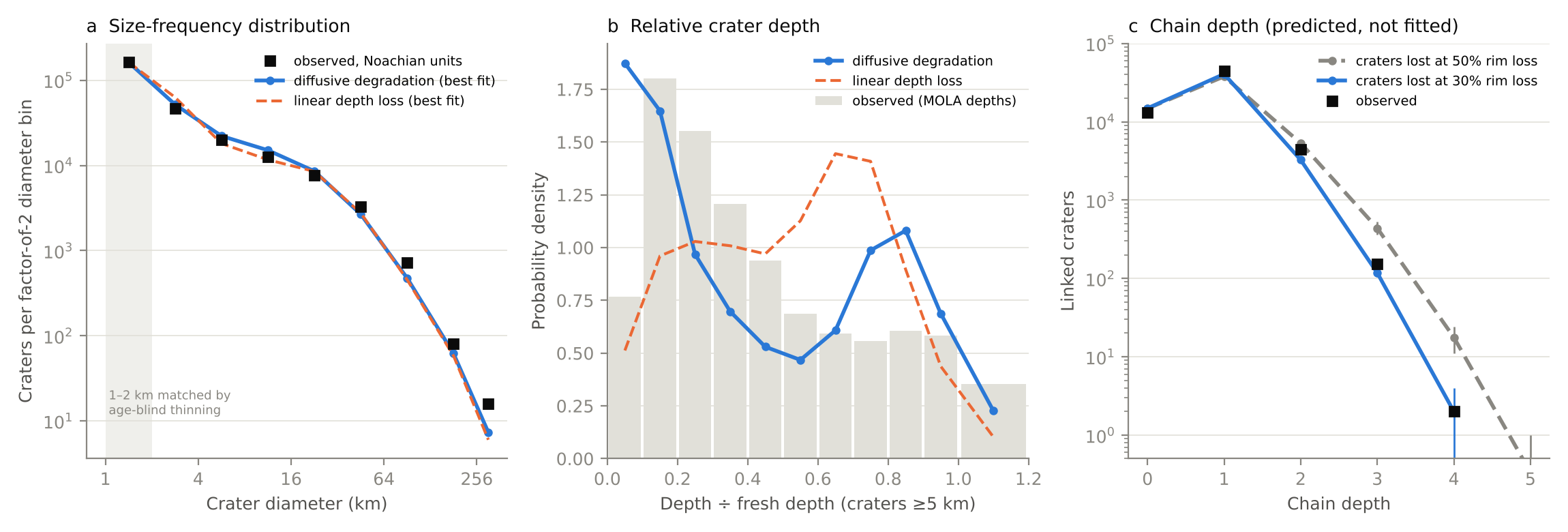
Figure 9. Degradation model fitted to craters on Noachian units. (a) Size-frequency distribution in factor-of-2 bins; the 1–2 km bin is thinned to the observed count and excluded from the fit. (b) Depth divided by fresh depth for craters ≥5 km, with depths measured on MOLA topography. (c) Chain depth predicted by the fitted model for craters lost at 50% and 30% rim loss; the graph was not used in the fit. Blue: diffusive degradation. Orange dashed: constant depth loss. Bars span three realizations.
Misfits. Four observations do not match the model. First, the model places 19% of craters ≥5 km below q = 0.1 and 21% between q = 0.7 and 0.9, against 8% and 12% observed, and it misses the observed peak at q = 0.1–0.3 (Figure 9b). A single diffusivity with an abrupt drop at 3.7 Ga cannot produce that peak; a gradual decline in rate, or infill that depends on more than crater size, might. Second, the excess of 1–2 km craters may reflect incompleteness of the catalog near its 1 km limit or faster removal of small craters than diffusion predicts. Third, the model gives 1,844–2,028 craters with two older neighbors and 30–37 with three, against 4,035 and 232 observed. Random impact positions may underrepresent clustered craters, such as secondary crater fields; we have not tested this. Fourth, on Hesperian units we modeled resurfacing as one deposit laid on the Noachian surface. The best single deposit is 0.8 km thick and emplaced at 3.6 Ga, and it overpredicts craters 16–128 km across by a factor of 2–3, so a single deposit of uniform thickness is too simple for these units.
9. Discussion and outlook
The graph gives 83,370 Martian craters ordinal age constraints derived only from geometry and rim preservation. For any linked crater it returns the full set of craters known to be older and younger, and for any region it returns the superposition sequence without new mapping. Because the edges are independent of crater degradation classes and crater-count model ages, they can be used to test both (Section 6). The distribution of chain depths also constrains how craters are erased, and together with a cratering model it gives crater degradation rates (Sections 7 and 8).
Five limits apply to this version.
- Fragmentation. Superposition orders only craters that touch, so the graph consists of 14,415 clusters. A single global sequence requires relations that span distance, such as ejecta superposition, embayment by dated units, or crater-count model ages assigned to whole clusters.
- Ejecta-zone pairs. The pair search found 291,097 pairs in which the smaller crater lies within one radius of the larger crater’s rim, on its continuous ejecta. Whether the smaller crater sits on that ejecta or is buried by it can be read only from imagery. These pairs outnumber all current edges by a factor of 3.75.
- Unoriented overlaps. Of the 26,711 overlapping pairs, 10,529 remain unoriented: 10,510 that neither test decides and 19 on which the tests disagree.
- Small craters. Craters smaller than 3 km are oriented by the rim-arc test alone, because MOLA does not resolve their rims. The CTX check supports those calls in 19 of 21 cases, but the sample is small.
- Missing basins. The largest crater in the catalog is 1,088 km across, so Hellas, Argyre, Isidis, and Utopia are absent, and the craters inside them are not linked to them.
Host geologic units are recorded as crater attributes and not as edges. A crater’s host unit bounds the crater’s age only where the crater is superposed on the unit rather than embayed by it, and the global map does not record which case applies.
Four extensions follow directly. An image classifier trained on CTX and THEMIS views of the 15,686 oriented overlap pairs could orient the unoriented overlaps and the ejecta-zone pairs. The 200 m/pixel HRSC–MOLA blended topography (Fergason et al., 2018) would extend the rim-continuity test to craters near 1.5 km. The large basins can be added as nodes from published rim definitions. Automated counts of small craters on CTX images, which have been used to date individual large Martian craters (Lagain et al., 2021), would give each host crater many more counted craters than the 1 km catalog provides and narrow the intervals of the sequence model in Section 6.4.
Data and code availability
The edge list, the crater table with graph metrics, the GraphML file, and the pair-level evidence are archived on Zenodo (concept DOI 10.5281/zenodo.23675713). The pipeline code (Python; NumPy, pandas, SciPy, NetworkX, GeoPandas), the code for the analyses in Sections 6–8, and the interactive map explorer are at github.com/michael-s-phillips/mars-crater-graph. The explorer is a self-contained web page that runs at michael-s-phillips.github.io/mars-crater-graph. The graph pipeline runs in about two minutes on a laptop. Input data are public: the Robbins and Hynek (2012) crater database, including the MOLA depths of its original release; the MOLA gridded topography from the NASA Planetary Data System Geosciences Node; the THEMIS daytime infrared global mosaic (Edwards et al., 2011); the geologic map of Tanaka et al. (2014) from the U.S. Geological Survey; and the CTX mosaic of Dickson et al. (2024).
How this was made
Michael Phillips posed the question, chose the data sources, set the scope of each analysis, and asked the questions that led to Sections 6–8: what the graph implies for crater-count ages, why chains are no more than four relations deep, and whether chain depth could measure erosion rates. Claude (Anthropic), an AI model working in the Cowork mode of the Claude desktop app, wrote the code, ran the analyses and simulations, made the figures, and drafted the text over 26–27 October 2026. Phillips decided what to pursue as each result came in.
Several first results changed on checking. The interior density ratio in Section 6.2 fell from 1.76 to 1.66 once the younger crater of each pair was removed from the older crater’s count. The first explanation of short chains used the total crater coverage, which matched the observations by coincidence; the coverage by craters smaller than the host applies (Section 7). Claude also made the blind visual calls on CTX images in Section 4, and a repeat of that check by a person is planned. References were checked against publisher or repository pages where possible.
Acknowledgments
CTX mosaic data credit: NASA/JPL/MSSS/The Murray Lab. THEMIS daytime infrared mosaic: NASA/JPL/Arizona State University.
References
- Aho, A. V., Garey, M. R., & Ullman, J. D. (1972). The transitive reduction of a directed graph. SIAM Journal on Computing, 1(2), 131–137. doi:10.1137/0201008
- Barlow, N. G., Boyce, J. M., Costard, F. M., Craddock, R. A., Garvin, J. B., Sakimoto, S. E. H., Kuzmin, R. O., Roddy, D. J., & Soderblom, L. A. (2000). Standardizing the nomenclature of Martian impact crater ejecta morphologies. Journal of Geophysical Research, 105(E11), 26733–26738. doi:10.1029/2000JE001258
- Bronk Ramsey, C. (2009). Bayesian analysis of radiocarbon dates. Radiocarbon, 51(1), 337–360. doi:10.1017/S0033822200033865
- Buck, C. E., Kenworthy, J. B., Litton, C. D., & Smith, A. F. M. (1991). Combining archaeological and radiocarbon information: A Bayesian approach to calibration. Antiquity, 65(249), 808–821. doi:10.1017/S0003598X00080534
- Christensen, P. R., et al. (2004). The Thermal Emission Imaging System (THEMIS) for the Mars 2001 Odyssey mission. Space Science Reviews, 110, 85–130. doi:10.1023/B:SPAC.0000021008.16305.94
- Dickson, J. L., Ehlmann, B. L., Kerber, L., & Fassett, C. I. (2024). The global Context Camera (CTX) mosaic of Mars: A product of information-preserving image data processing. Earth and Space Science, 11(7). doi:10.1029/2024EA003555
- Edwards, C. S., Nowicki, K. J., Christensen, P. R., Hill, J., Gorelick, N., & Murray, K. (2011). Mosaicking of global planetary image datasets: 1. Techniques and data processing for Thermal Emission Imaging System (THEMIS) multi-spectral data. Journal of Geophysical Research, 116, E10008. doi:10.1029/2010JE003755
- Fassett, C. I., Head, J. W., Kadish, S. J., Mazarico, E., Neumann, G. A., Smith, D. E., & Zuber, M. T. (2012). Lunar impact basins: Stratigraphy, sequence and ages from superposed impact crater populations measured from Lunar Orbiter Laser Altimeter (LOLA) data. Journal of Geophysical Research, 117, E00H06. doi:10.1029/2011JE003951
- Fergason, R. L., Hare, T. M., & Laura, J. (2018). HRSC and MOLA blended digital elevation model at 200 m v2. Astrogeology PDS Annex, U.S. Geological Survey. Data page
- Golombek, M. P., Grant, J. A., Crumpler, L. S., Greeley, R., Arvidson, R. E., Bell, J. F., III, Weitz, C. M., Sullivan, R., Christensen, P. R., Soderblom, L. A., & Squyres, S. W. (2006). Erosion rates at the Mars Exploration Rover landing sites and long-term climate change on Mars. Journal of Geophysical Research, 111, E12S10. doi:10.1029/2006JE002754
- Hagberg, A. A., Schult, D. A., & Swart, P. J. (2008). Exploring network structure, dynamics, and function using NetworkX. In Proceedings of the 7th Python in Science Conference (SciPy 2008), 11–15.
- Harris, E. C. (1979). The laws of archaeological stratigraphy. World Archaeology, 11(1), 111–117. doi:10.1080/00438243.1979.9979753
- Hartmann, W. K., & Neukum, G. (2001). Cratering chronology and the evolution of Mars. Space Science Reviews, 96, 165–194. doi:10.1023/A:1011945222010
- Ivanov, B. A. (2001). Mars/Moon cratering rate ratio estimates. Space Science Reviews, 96, 87–104. doi:10.1023/A:1011941121102
- Kneissl, T., Michael, G. G., & Schmedemann, N. (2016). Treatment of non-sparse cratering in planetary surface dating. Icarus, 277, 187–195. doi:10.1016/j.icarus.2016.05.015
- Lagain, A., Servis, K., Benedix, G. K., Norman, C., Anderson, S., & Bland, P. A. (2021). Model age derivation of large Martian impact craters, using automatic crater counting methods. Earth and Space Science, 8(2), e2020EA001598. doi:10.1029/2020EA001598
- Malin, M. C., et al. (2007). Context Camera Investigation on board the Mars Reconnaissance Orbiter. Journal of Geophysical Research, 112, E05S04. doi:10.1029/2006JE002808
- Mangold, N., Adeli, S., Conway, S., Ansan, V., & Langlais, B. (2012). A chronology of early Mars climatic evolution from impact crater degradation. Journal of Geophysical Research, 117, E04003. doi:10.1029/2011JE004005
- McGetchin, T. R., Settle, M., & Head, J. W. (1973). Radial thickness variation in impact crater ejecta: Implications for lunar basin deposits. Earth and Planetary Science Letters, 20(2), 226–236. doi:10.1016/0012-821X(73)90162-3
- Michael, G. G. (2013). Planetary surface dating from crater size–frequency distribution measurements: Multiple resurfacing episodes and differential isochron fitting. Icarus, 226(1), 885–890. doi:10.1016/j.icarus.2013.07.004
- Michael, G. G., & Neukum, G. (2010). Planetary surface dating from crater size–frequency distribution measurements: Partial resurfacing events and statistical age uncertainty. Earth and Planetary Science Letters, 294, 223–229. doi:10.1016/j.epsl.2009.12.041
- Richardson, J. E. (2009). Cratering saturation and equilibrium: A new model looks at an old problem. Icarus, 204(2), 697–715. doi:10.1016/j.icarus.2009.07.029
- Robbins, S. J., & Hynek, B. M. (2012). A new global database of Mars impact craters ≥1 km: 1. Database creation, properties, and parameters. Journal of Geophysical Research, 117, E05004. doi:10.1029/2011JE003966
- Robbins, S. J., Hynek, B. M., Lillis, R. J., & Bottke, W. F. (2013). Large impact crater histories of Mars: The effect of different model crater age techniques. Icarus, 225(1), 173–184. doi:10.1016/j.icarus.2013.03.019
- Shoemaker, E. M., & Hackman, R. J. (1962). Stratigraphic basis for a lunar time scale. In Z. Kopal & Z. K. Mikhailov (Eds.), The Moon (IAU Symposium 14), 289–300. Academic Press. NTRS record
- Smith, D. E., et al. (2001). Mars Orbiter Laser Altimeter: Experiment summary after the first year of global mapping of Mars. Journal of Geophysical Research, 106(E10), 23689–23722. doi:10.1029/2000JE001364
- Tanaka, K. L. (1986). The stratigraphy of Mars. Journal of Geophysical Research, 91(B13), E139–E158. doi:10.1029/JB091iB13p0E139
- Tanaka, K. L., Skinner, J. A., Jr., Dohm, J. M., Irwin, R. P., III, Kolb, E. J., Fortezzo, C. M., Platz, T., Michael, G. G., & Hare, T. M. (2014). Geologic map of Mars. U.S. Geological Survey Scientific Investigations Map 3292. doi:10.3133/sim3292
- Wilhelms, D. E. (1987). The geologic history of the Moon. U.S. Geological Survey Professional Paper 1348. doi:10.3133/pp1348